
Change The Case In Rows Or Columns In Excel
Now that you have listed your entire DVD or CD collection and added the list of artists, you notice that some entries are capitalized, and some aren’t. The thought of going through 400 or 500 lines with multiple columns is daunting but don’t worry, Excel has you covered.
Unlike Word, Excel does not have a “Change Case” button. But then again, in Word, every entry is not in its own individual cell as they are in Excel.
However, Excel does have text functions similar to its number functions. Functions are “built-in” formulas designed to perform specific tasks, in this instance, converting text cases. Using the =PROPER, =LOWER, =UPPER functions you can let Excel change the case in individual cells, columns, or rows.
So instead of having an entry shown in the top row, you can easily change it to Title Case as shown in the middle row, or change the video title to all caps as shown in the bottom row.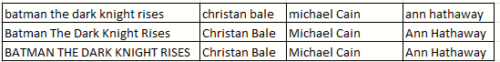
The method of changing cases in Excel is not initially obvious but once you understand the process it is straightforward.
Title Case
Whenever a title or published work is printed, it is normally printed in “title case”. When using title case, all words except minor words are capitalized Normally headlines or published works use title case when writing the name. To use Title Case in Excel, you would use the =PROPER function.
Changing Case In A Column
The first step for changing the case for a column is to create a temporary column next to the column you wish to convert. Do this by right-clicking on a column and selecting “Insert”
To change the case to Title case in the first column, you need to use the =PROPER function. In this case, you would enter the formula =PROPER(A2) cell B2. The formula instructs the text in cell A2 to enter the Title Case in the corresponding row.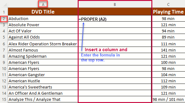
Once the formula is entered, the Title case will appear in cell B2. Double-click on the square at the bottom right of the selected cell and it will auto-populate the entire column with the changed case. 
To complete the change, select the values in the new column (B) and copy them to the clipboard. Right-click on cell A2 and choose Paste “Values”. It will be the second option when you right-click. This allows you to copy the actual values of the cell and not the formula. Once completed, delete the B column and everything is as it should be.
You are not restricted to only Title cases. If you wanted to have the DVD title displayed in all caps, you just need to enter a different formula. =UPPER(A2) or if you wanted to have the text to be displayed in all lowercase, you would use the formula =LOWER(A2).
Changing Data In Rows
If the data, you have in Excel is in a row, the process is similar. Enter the formula in the row beneath the row you wish to change and below it would be =PROPER(A1). Press Enter and when the correct case appears, select the box and drag it to the right until the entire row has been changed.
Summary
You don’t need to understand formulas in Excel to make these changes. Just knowing that entire columns and rows can be changed with these three formulas to match your needs makes it a simple chore.
—
Sometimes my EXCEL editing thinks it knows what I want ‘better than me’ and after I’m done, it will change some of my typing. For example, often when Excel sees I have an at-sign symbol (@), it will assume I meant an email and will change its color from black to blue, underline it (as if I intended it to be hypertext), and if I click on it it will open Outlook and insert what I just typed as the TO address in the email?!?
Is there an Excel setting that is set somewhere requesting Excel to make me live with this unintended consequence?!?
Nice article, by the way!
Dan
Hi Dan, Yes, there are a couple of ways to do this. Personally, I prefer the first method. 1. When I type an @ symbol and don’t wish it to be shown as an internet address and turn blue. I right -click on the item I typed and click on Remove Hyperlink, and it will just revert to regular text. You can also click any grouping of cells or use Control A and then right click and select Remove Hyperlink.
2. You can also Turn off automatic hyperlinks by choosing File > Option > Proofing > Select the “AutoFormat As You Type” tab and uncheck – “Internet and network paths with hyperlinks”
The second option does not remove existing hyperlinks or copied hyperlinks; it is strictly for when you type. None of the text you type will appear as a hyperlink.
Thanks, Jim.
There are additional similar issues I have but I’ll explore the Options panel you suggested to see if I can find their answers.
Dan