
There are many reasons why you might want to control a user’s input in a worksheet. My number one reason is that it saves time and keystrokes and everyone knows how much I love that!
Another reason is that it will limit the choices and you will then be certain to get the data that you require and will not have to wade through a lot of information you were not looking for or typos, etc.
The bottom line is that you want things to be as consistent as possible in your worksheet and you want to be efficient and save time. It also helps that Excel makes it very easy to create your own custom drop-down list.
Follow the steps below to learn how:
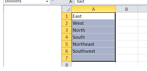
- Key in the list of values you would like to use for your drop-down list someplace in your workbook (on a worksheet other than your input sheet).
- Select the range of cells where you have just entered your list of values and key in a name for your list in the Name box, (the area to the left of your Formula Bar), beginning with a letter and no spaces.
- Click Enter.
- Select the range of cells in your worksheet where you would like your drop-down list to appear.
- On the Data tab of your Ribbon, in the Data Tools group, click Data Validation.
- On the Settings tab, from the allow drop-down menu, select List.
- In the Source box, enter an equal sign ( = ) and the name you created for your list, above.
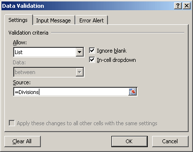
- Click OK.
- Now, when you click any cell in your input range, the drop-down arrow will appear to the right of that cell.
You can now select a value from the drop-down list you have created.
Life will be a lot easier for you now that you have this handy little tool in your arsenal.
—