There are two ways to work with dates in Excel, the hard way where you do all the work or the easy way where Excel does all the work for you.
If you work with monthly sheets e.g. Jan, Feb, etc. then this tutorial may be of some help to you.
I use this for my work time-sheet but it can be used for anything that you document on a daily basis in Excel.
On the first sheet I have my name and the year I want the book to use.
The first point to note is that you need only enter a year and all the dates for the rest of that year will be filled in the appropriate cells. This cell must not be formatted in the date format! Set the formatting to Number and the decimal places to 0.
To make things easier for me to explain I will assume you will have a front or start sheet where you would enter things like your name, the year, etc.
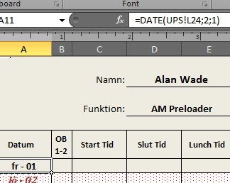
On the second sheet which I called January in which any cell you choose to be Jan 1st use the formula: =DATE(Sheet1!L24;1;1)
This is telling Excel to read the number in cell L24 on the first sheet as a year and then start at the first day of the first month – Jan 1st.
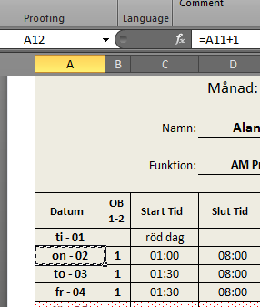
On my work sheet this happens to be cell A11 yours could be A1, etc.
In the cell below it type the =A11+1 using your own cell number of course.
Highlight the cell and press Ctrl+C to copy the formula then highlight the next 29 cells below it and press Enter to paste the formula into them.
Highlight all 31 cells then right click and select Format Cells.
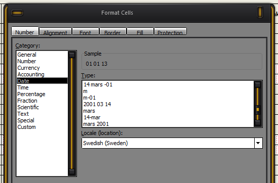
Choose Date as the format option and then one of the many date formats that suits you.
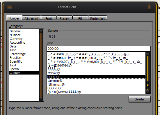
As I only wanted the day and date I chose Custom and then the DDD DD format which gives me the first two letters of the day and the day number, as I said, make whichever choice suits you.
The first thing to notice is that the dates go down to 31 which is all well and good for January but no good for February.
To correct this highlight the third from last cell i.e. what would be the 29th of the month.
In that cell delete the formula and replace it with =IF(MONTH(A38+1)>MONTH(A38);””;A38+1) take note that A38 is the cell that I have due to the fact that the first day of the month is in cell A11 in my work sheet so A38 is the 28th day, change this cell number to suit your work sheet.
In the next cell down – effectively the 30th day of the month use this formula again substituting the cell number in your work sheet: =IF(MONTH(A38+2)>MONTH(A38);””;A39+1). Note the first part of the formula points to A38+2 and the last part points to A39+1 in my sheet.
Then in the last cell use the formula =IF(MONTH(A38+3)>MONTH(A38);””;A40+1) again taking note of the cell references.
Now as you have entered the formula =DATE(Sheet1!L24;1;1) where L24 points to the cell with your year in it, you have the dates for January, if you want to test February then change the formula in the first cell to =DATE(Sheet1!L24;2;1) which is telling Excel to start at Feb 1st and you will see that the last three cells are blank as they should be.
So far so good!
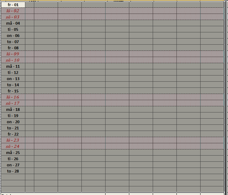
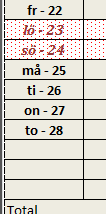
As you can see the weekends in my worksheet are highlighted in a different colour and in italics. You can achieve this through conditional formatting.
First make sure you have the Home tab ribbon chosen then highlight all the cells from the 1st down to 31st of the month including all the cells across the page that you want to show up as a weekend.
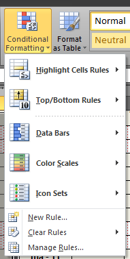
Now click on Conditional formatting and select New Rule.
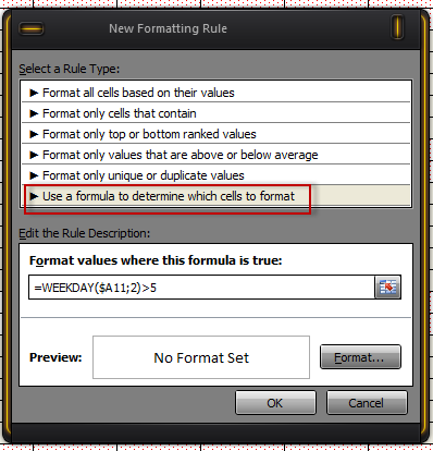
Click on the ‘Use a formula to determine which cells to format’ option and use this formula in the Value box: =WEEKDAY($A11;2)>5 again change the cell number from A11 to whatever is the first of the month in your sheet.
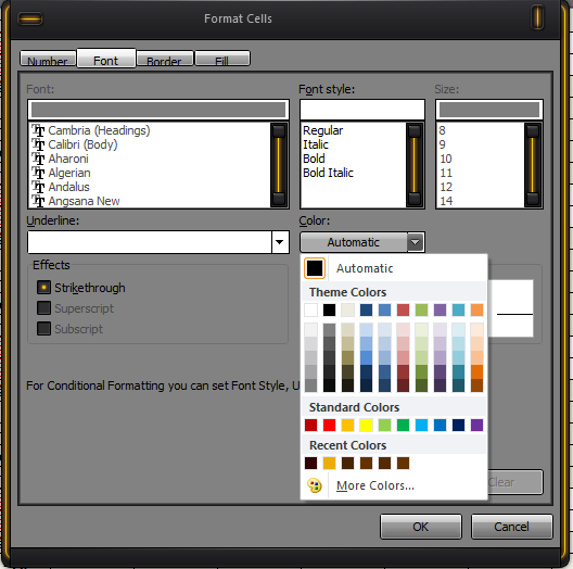
Click on Format and now you can format the weekend cells to whatever suits your taste.
To change the font colour make sure the font tab is selected and click on the colour box then on your desired colour.
To fill the cells with a pattern click on the Fill tab then make your choices.
Click on OK then OK again and you should now have highlighted weekends.
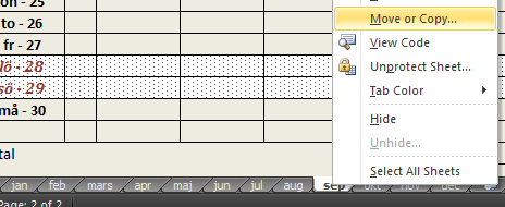
If you want to make a year book, i.e. a different sheet for each month, then right click on your sheet tab at the bottom then on Move or Copy.
In the window that opens check the Create a Copy box then click OK. Rename the new sheet to what ever you want to call it – Feb for example.
Highlight the first of the month cell and change the formula as previously explained the next to last 1 to 2 and the cell reference L24 to the cell number that contains your year.
Do the same for each month you create e.g. March would be =DATE(Sheet1!L24;3;1) again assuming L24 is the cell on the first sheet that contains the year.
Once completed you can save the workbook as a template which can be used year after year.






Good article, unfortunately the 2 letter month abbreviations in Swedish (?) in the screen captures is a little jarring.
The 2 2 letters are for the days of the week, unfortunately although I changed the UI to English the days and months remained in Swedish. But I am sure you got the general idea.
The last 3 days of February didn’t come out blank for me. I got the first 3 days of March instead.
Tony, post your formula for one of the three days and I will look at it for you.
Formula for 29th January:
=IF(MONTH(A28+1)>MONTH(A28),””,A28+1)
Copied to February didn’t show blank, rather it gives 1st March.
Ok, sorry its been a day or two.
On your worksheet for Feb does cell A28 correspond with the 28th Feb?
By that I mean is A1 the 1st of Feb?
Have all the cells in the range A1 to A31 (assuming A1 is the 1st of the month) been formatted to a date format?
P.S. Once you have checked the above, if you still cannot get it to work contact me using the the Contact link at the top of the page. If your worksheet dosnt contain sensitive data you can email a copy to me and I will look to see where it has gone wrong.
Looks like the semi-colons in this formula =DATE(Sheet1!L24;1;1) should be commas.