Transposing (i.e., swapping columns, rows, etc.) is an old trick in Excel and I am happy to report that it is still available to you in Excel 2013!
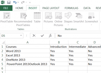
As you will see in my screenshot below, I have a worksheet in Excel that is vertical in orientation, using a column style.
- So go ahead, and create your own worksheet so you call follow along.
- Now we can move forward and change the same worksheet into a horizontal row style.
- From your worksheet, select the cells you would like to change.
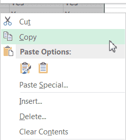
- Now, right-click and select Copy.
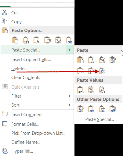
- Next, right-click in any empty cell and select Paste Options | Transpose as shown below.
- One of the special features of Excel 2013 is it will show you a preview of what your paste will look like before confirming the action.
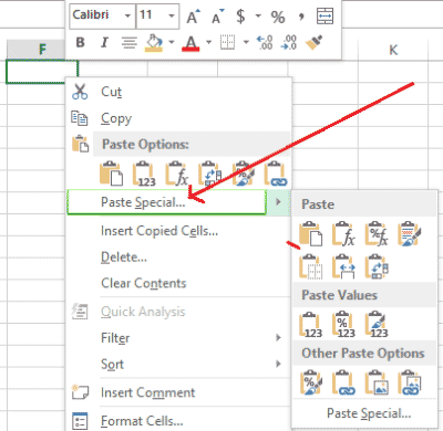
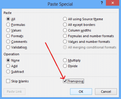
- If you do not see that, as an alternative step, you can right-click an empty cell and select Paste Special.
- You can now from it’s window, check the Transpose box.
- Click OK.
You will now see your data has been transposed to a new layout style.

Thanks Carol for this article I think excel is a great tool. Sometimes I need a little help figuring out where they move features when they change versions. Plus you know how to explain it clearly. Keep them coming 🙂