For decades, anyone working with text data in Excel has been limited to the same old functions for separating or parsing text strings. But recently, Excel added three new dynamic array text functions. And they are awesome! The new functions are designed to manipulate text data that have delimiters. The three new functions are TEXTBEFORE, TEXTAFTER, and TEXTSPLIT.
TEXTBEFORE And TEXTAFTER Functions
The TEXTBEFORE and TEXTAFTER functions are similar and use a similar syntax. The TEXTBEFORE function extracts the text from a string that occurs before the specified delimiter. The TEXTAFTER function extracts the text from a string that occurs after the specified delimiter.
Syntax
=TEXTBEFORE(text,delimiter,[instance_num], [match_mode], [match_end], [if_not_found])
=TEXTAFTER(text,delimiter,[instance_num], [match_mode], [match_end], [if_not_found])
Text The text you are searching for. Required.
Delimiter The text that marks the point after which you want to extract. Required.
instance_num The instance of the delimiter. If you have multiple instances of the same delimiter, choose the instance other than the first one. A negative number starts searching text from the end. Optional.
match_mode Determines whether the text search is case-sensitive. Optional.
match_end Treats the end of the text as a delimiter. Optional.
if_not_found Value returned if no match is found. Optional.
Example
For example, suppose I had a simple list of names with some data separated by commas. I could use the Text to Columns tool to separate the data into columns. But that is a tool. It is not dynamic. To make it dynamic (the results update automatically as the source data changes), I need to put formulas in each column. Previously, I had to determine the location of the delimiter and the length of the text I wanted. It was tedious using a combination of the RIGHT, LEFT, and MID functions with LEN, SEARCH, FIND, SUBSTITUTE, or REPLACE. There are a few ways to do this, but here is one way I could have done it using the old functions. Imagine how cumbersome this could be with 40 or 50 columns!
Column B would be =LEFT($A2,(SEARCH(“,”,$A2)-1))
Column C would be =MID($A2, SEARCH(“,”,$A2) + 1, SEARCH(“,”,$A2,SEARCH(“,”,$A2)+1) – SEARCH(“,”,$A2) – 1)
Column D would be =MID($A2, FIND(“#”,SUBSTITUTE($A2,”,”,”#”,2))+1, FIND(“#”,SUBSTITUTE($A2,”,”,”#”,3)) – FIND(“#”,SUBSTITUTE($A2,”,”,”#”,2))-1)
Column E would be =MID($A2,(FIND(“/”, SUBSTITUTE($A2,”,”,”/”, LEN(A2)-LEN(SUBSTITUTE($A2,”,”,””))))+1),10000)

Using the new TEXTBEFORE and TEXTAFTER functions is much easier. Here is one way to do it now:
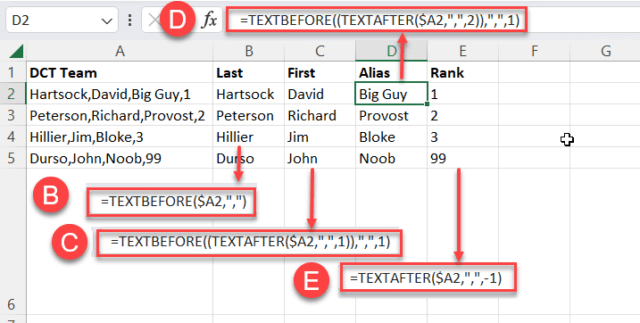
Column B would be =TEXTBEFORE($A2,”,”)
Column C would be =TEXTBEFORE((TEXTAFTER($A2,”,”,1)),”,”,1)
Column D would be =TEXTBEFORE((TEXTAFTER($A2,”,”,2)),”,”,1)
Column E would be =TEXTAFTER($A2,”,”,-1)

TEXTSPLIT Function
Syntax
The TEXTSPLIT function works similarly to the Text-to-Columns tool but in the form of formulas. It allows you to split across columns or down by rows.
=TEXTSPLIT(text,col_delimiter,[row_delimiter],[ignore_empty], [match_mode], [pad_with])
Text The text you want to split. Required.
col_delimiter This character will be treated as the column separator. Required
row_delimiter This character will be treated as the row separator. Optional.
ignore_empty TRUE to ignore consecutive delimiters. Defaults to FALSE, which creates an empty cell. Optional.
match_mode Determines whether the match is case-sensitive. Optional.
pad_with The value with which to pad the result. The default is #N/A. Optional.
TEXTSPLIT results in a spilled array. Therefore, all cells where the results will be returned must be empty. Otherwise, Excel will return an error.
Examples
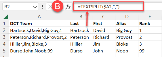
The TEXTSPLIT function is an improvement over Text to Columns because it is dynamic. Using the same example above, a simple list of names with data separated by commas is much easier with TEXTSPLIT. Here is how to do it.
Column B would be =TEXTSPLIT($A2,”,”)

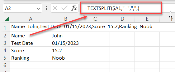
TEXTSPLIT can also split delimited data into rows. Here is an example that splits the data into a new column for each equal sign delimiter and a new row for each comma delimiter.

A final example is to use TEXTSPLIT to split the date into its various parts and put each into a column.

Bottom Line
For anyone working with data in Excel, splitting values into separate columns and rows is usually only a first step before performing data analysis or data conversions. The three new text functions TEXTBEFORE, TEXTAFTER, and TEXTSPLIT make this task much easier.
—
