
![]()
Suppose you had values in Column A of your worksheet and a list in Column B. There is a conditional format that makes any value in Column A turn red if it is also in Column B and you want to sort or filter by that result and it is not terribly difficult to do.
All you have to do is set up your data and your conditional formats to your liking.
Follow the steps below to learn how to set up your sorting:
- Select all the cells you would like included in the sort
- Display the Data tab of your Ribbon
- Click the Sort tool to open the dialog box
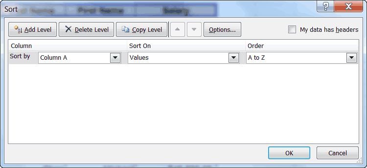
- Using the Sort By drop-down list, select Column A, where your conditional formatting has been applied
- Using the Sort On drop-down list, select Font Color
- Using the Order drop-down list under Order, select the color you would like to sort by. In this instance it would be red
- Using the second drop-down list under Order, specify whether you want the red font cells to be on top or on the bottom of the list
- Click OK
That’s all there is to it. If the colors of your cells change because of conditional formatting, you can resort your table and you will have no problems.
Should you want to filter by the colors you can easily do that using an AutoFilter.
Follow the steps below to learn how:
- Turn on AutoFiltering by clicking on the Data tab of your Ribbon
- In the Sort and Filter group, select Filter
- Click the down-arrow at the top of Column A and you will see many options available to you
- Select Filter by Color to display a list of the colors that are in your column
- Select the color that you would like displayed. Usually one would select Automatic
—