A client wrote to me recently with this problem: She had a worksheet with about six thousand rows (yes, those do exist!).
At the very top of her worksheet there is a graph based on her data with the data starting at row 50. The top 50 rows are frozen so she can always see her graph and column headings
When she scrolls through her data and reaches row number 1000, however, the row labels become wider and force the graph to be redrawn. The redrawing in turn, slows down her scrolling. She needs to find a way to set the width for her row labels so they will be wide enough to accommodate the four digits necessary for the upper rows.
There are more than one way in which to work on this, the first of which being to turn off the row and column headings.
Follow the steps below to learn how:
- Click File | Options.
- At the left of the resulting dialog box, click Advanced.
- Scroll down until you see the Display Options for this Worksheet section.
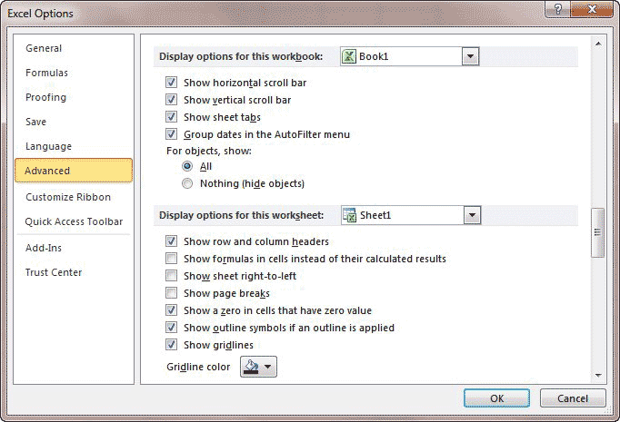
- Make certain the Show Row and Column Headers box is selected. If it is clear, then the header area will not be displayed.
- Click OK.
It is now a non-issue because Excel will not display the row headers at the left of her screen. If you really want to have an indication as to the row number, you could always insert a blank column A and then insert numbers to represent your row numbers. You column can be as wide as you need so there will not be any redrawing when you scroll.
Another method would be to actually start her data and graph below row 1000. She could insert enough blank rows above her graph and data to move them down into the four digit range and then hide rows 1 through 999.