


Degree of difficulty explanation: Windows Tips DOD (degree of Difficulty) = 1
How To Freeze Panes In Excel
Whenever you have either several columns of data or more likely several rows of data, it can be difficult to remember where you are when you have to scroll through the data, and you no longer have the header row visible or the first column available to reference.
Fortunately, Excel gives you several options to freeze the Top and Side Panes. In addition, they can be used in combination. Another handy option is to freeze several panes that you want to be always visible.
Freezing The Top Header
I want to see the header no matter how far down I scroll.
The simplest option is to freeze the Header. In the search area at the top of Office enter freeze. 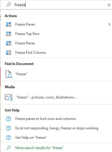
A drop-down menu will appear giving you the options you will need. Clicking the first “Freeze Panes” option will open a fly-out menu. 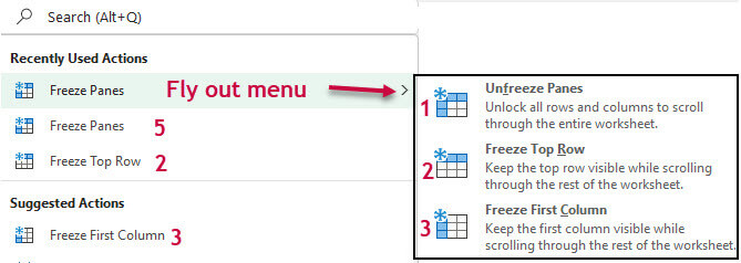


It would be difficult for me to enter weekly data for a player if their name disappeared as I scrolled to week 8, so if freezing just the left column is what you want, click on option 3.
Selecting either option 2 or 3 will cancel the other. In other words, if you already have the header frozen, then freezing the left column will remove the freeze on the header. That only happens if you use options 2 or 3 but there is another way to freeze any panes you want.
Unfreeze All Frozen Panes
If you make a mistake don’t worry – clicking on option 1 in the fly-out menu at any time will erase all frozen panes.
Freezing Both Columns And Rows
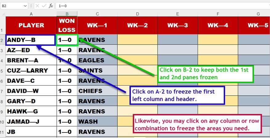
For my purposes, I want to freeze the header and the first two columns. This way whenever I scroll across or down, they are always visible. I can enter this week’s data and know I have the correct player and week combination.
Seeing The Top And Bottom Rows
What if you need to see the top and bottom rows when you are doing something like number totals? Freezing the top and bottom would be difficult but there is a way nicely explained in Carol Bratt’s article for Office 10. The newer versions of Office, as well as Microsoft 365, are very similar. If you are using Office 10 please check out her article. Newer versions are almost identical. In the top Tool Bar, click on View>New Window. This will open an additional window of your spreadsheet. You can Click on Arrange All to align them horizontally. An even easier way is to click somewhere in the middle of your spreadsheet and click on Split. This will effectively divide your spreadsheet into two sections and you can view the top and bottom portions with ease. 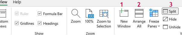
Summary
In the example above, I only needed to choose B-2 to freeze the top header and the two left columns but you are not limited to the number of top rows or the number of left columns you wish to freeze. If your chart requires the first three top rows to remain frozen and the first three columns no problem. Just select D-4 when freezing the panes.
—

