You can create a simple list for your users to select from in your worksheet. This will greatly reduce errors because you are limiting input from the user’s keyboard and makes things quick and easy for them as well. Everyone loves quick and easy, right? I know I do!
You only need two things for your list and they are data and an entry cell.
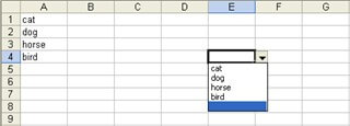
Below is an example of a simple drop-down list in an Excel worksheet. You can see how users can click the drop-down arrow to display a list of items stored in A2:A4. Should a user attempt to enter something that does not appear in that list, Excel will, by default, reject it.
Add A Drop-Menu
Follow the steps below to learn how to add this drop-down list to your worksheet:
- Create the list in cells A1:A4.
- Select cell E3, the data entry cell.
- Click the Data tab.
- Click the Data Validation option in the Data Tools group.
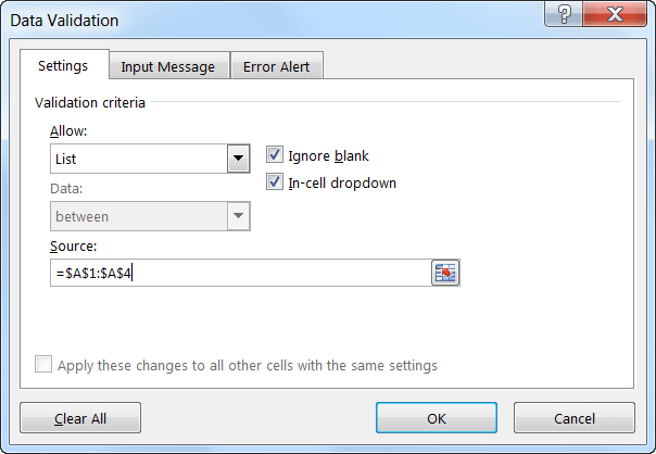
- From the Allow options drop-down, select List.
- Click the Source control and select cells A1:A4.
- Alternatively, you can simply enter the reference =$A$1:$A$4. Be certain the In-cell drop down option is selected. If you deselect this option, Excel will still force users to only enter list values, but it will not present a drop-down list.
- Click OK.
Your users can now use the drop-down and select an item to enter as a value in cell E3 and E3 equals the selected value.
It should be noted that the drop-down arrow will only be visible when the cell is active. To make it easier to use, you could apply a fill color or border to the cell.
—


